해당 글은 Algorithms. by S. Dasgupta, C.H. Papadimitriou, and U.V. Vazirani 를 정리한 스터디 노트입니다.

Chapter 5 Greedy algorithms

• 탐욕 알고리즘
  • 순간 순간마다 해결책을 선택하는 알고리즘
  • 특히 the most obvious & immediate benefit 을 가지는 방법을 선택
• 엄청난 양의 계산양이 발생할 수 있어도, 최적화하는 방법인 경우도 많다.

5.1 Minimum spanning trees

문제 상황

• 여러 대의 컴퓨터와 그것들을 서로 연결할 네트워크를 찾고 있음
• 그래프 문제로 해석한다면 → 각 노드가 컴퓨터 + 엣지가 연결관계
• 이 때, 엣지에는 유지비용으로 edge’s weight로 반영됨
• 최소한의 비용으로 가능한 네트워크는?

Property 1 : Removing a cycle edge cannot disconnect a graph (자명)

• 결국 문제 상황에서 원하는 네트워크 구조는 트리 구조임을 알 수 있다.
  • tree = connected & acylic & undirected graph
• 특히, total weight가 가장 낮은 트리를 minimum spanning tree 라고 부름

Formal Definition (finding MST)

• Input : An undirected graph $G = (V,E); \text{ edge weights } w_e.$

• Output : A tree $T = (V,E’), \text{ with } E’ \subseteq E, \text{ that minimizes }$

  \[\text{weight(T)}=\sum_{e \in E'}{w_e}\]

5.1.1 A greedy approach

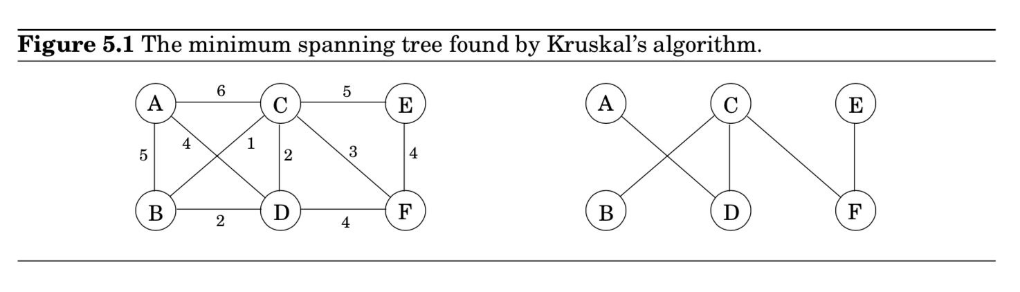
Kruskal의 m.s.t 알고리즘

• empty graph에서 시작해서 아래와 같은 룰에 의해 $E$로부터 추가될 엣지를 선택
• Repeatedly add the next lightest edge that doesn't produce a cycle
• 쉽게 말하면, 매순간마다 다음과 같은 선택을 한다는 뜻입니다.
  • avoid cycles
  • picks cheapest edge
• 탐욕 알고리즘 과정이라고 볼 수 있습니다.

• 빈 그래프에서 시작
• edge들을 weight순으로 오름차순 정렬
• Cycle 피하면서 edge 선택
  • $B-C$ 연결 → $C-D$ 연결 → $B-D$ 연결하지 않음 → $C-F$ 연결 …

Kruskal 방법의 정합성은 특정 cut property로부터 얻을 수 있음
사실, 이 cut property로부터 다른 많은 MST 알고리즘들을 justify할 수 있음

Property 2 : A tree on $n$ nodes has $n-1$ edges.

• 빈 그래프에서 하나씩 엣지를 추가하는 과정으로 보일 수 있음
  • 빈 그래프 = $n$ 개의 노드들이 서로 disconnected = 각 노드들 자체가 connected componenet
  • 엣지를 추가할 때마다, 하나씩 merge되므로 트리가 완성되기 위해서 총 $n-1$ 개의 엣지가 필요
• 특정 엣지 {u,v}가 연결된다는 것
  => u,v 노드는 분리된 connected components에 각각 놓여져 있다는 것임
  (만약, 그 사이에 path가 있었다면 uv에 의해 cycle을 만드는 결과가 나올 것이기 때문)
• 이렇게 하나의 엣지를 추가함으로써 connected components의 총 개수를 하나씩 줄여나가는 것임
• 계속 반복하면서, $n$개의 components들은 마지막 1개로 통합될 것이고, 이는 $n-1$ 엣지들이 추가된다는 뜻임

Property 3 : Any connected, undirected graph $G=(V, E)$ with $|E|=|V|-1$ is a tree.

• $G$가 acyclic임을 보이기만 하면 끝
  • do the following iterative procedure : 그래프에 cycle 존재할 경우, 해당 cycle 내의 edge를 제거함
  • $G’ = (V, E’), E’ \subseteq E, \text{ s.t. acyclic}$ 라는 그래프가 되는순간 process terminates
  • By Property 1, $G’$ is also connected.
  • 따라서, $G’$은 Tree이므로 Property 2에 의해 $|E’|=|V|-1$
  • $E’=E$ 이므로, 즉 어떤 엣지도 제거되지 않았다는 뜻임
  • 이 뜻은, $G$ 자체가 이미 cycle이 없다는 뜻 = acyclic
• 이 성질에 의해, 어떤 connected graph의 edge 수를 세서 tree인지 아닌지 파악할 수 있음

Property 4 : An undirected graph is a tree iff there is a unique path between any pair of nodes.

• $(\Rightarrow)$ 트리에서 어떤 두 노드 사이는 오직 하나의 path만 존재한다.
  • proof of Contradiction
• $(\Leftarrow)$ connected & acyclic임을 보이면 끝.
  • path가 항상 존재한다는 것은 모두 connected라는 뜻
  • 그 path가 unique하다는 것은 acyclic이라는 뜻
    • cyclic이면 두 노드 사이 path가 2개 존재한 뜻이므로

5.1.2 The cut property

MST를 만드는 과정에 있어서, 이미 몇가지 edges을 선택했고 올바른 방향으로 진행하고 있는 중이다. 어떤 edge를 다음에 추가할 수 있을까?

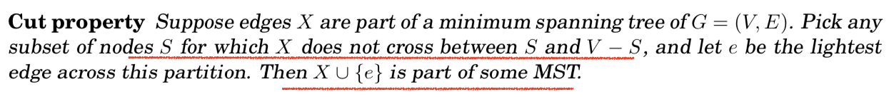
• $cut$ : 노드들을 partitions into two groups, $S \text{ and } V-S$
• 이 property가 설명하고 싶은 것 = 어떤 cut을 가로질러 가장 가벼운 edge를 추가하는 것은 항상 MST를 형성하는 방법임.

pf) Edges $X$를 MST인 $T$의 일부분이라고 하자.

• 1) 만약 새로운 edge $e$가 $T$의 일부분이면 증명할 필요가 없음.
• 2) 따라서, 새로운 edge $e$가 $T$에 없다고 가정하자.
  • $T$의 edge 하나를 바꿔서 $X \cup {e}$를 포함하는 새로운 MST $T’$를 construct함
    • $T$에 edge $e$ 추가.
    • $T$가 connected하기 때문에 이미 $e$의 끝점 사이에 path가 하나 존재함.
    • 즉, $e$를 추가함으로써 cycle을 만들었음
    • 이 cycle로 인해, $\text{the cut }(S, V-S)$을 가로지르는 다른 edge $e’$가 분명히 있음. (Figure 5.2)
    • 
    • 이 엣지를 제거함으로써, 새로운 $T’$을 얻게 됨. $T’ = T \cup {e} - {e’}$
    • Property 2와 3에 의해, $T’$은 tree임.
  • 게다가, $T’$은 MST임.
    • $\text{weight}(T’) = \text{weight}(T) + w(e) - w(e’)$
    • $e$와 $e’$ 모두 $S$ 와 $V-S$ 사이에 놓여진 edge지만, $e$가 더 가벼움 (=$w(e) \leq w(e’)$ )
    • 즉, $\text{weight}(T’) \leq \text{weight}(T)$.
    • $T$가 MST이므로, $\text{weight}(T’)=\text{weight}(T)$
    • $\therefore T’$ = MST

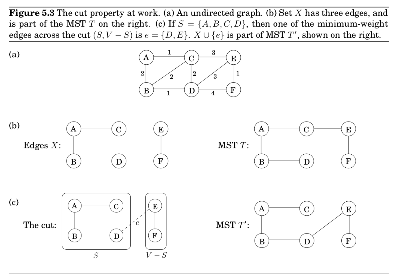
5.1.3 Kruskal’s algorithm

Justifying Kruskal’s algorithm

주어진 순간, 이미 선택한 edges는 하나의 partial solution을 형성하는데, 이 partial solution은 각각 tree 구조를 가진 connected components의 집합이라고 볼 수 있다. 새롭게 추가된 edge $e$는 이러한 components 중 특정 2개의 components $T_1$과 $T_2$ 사이를 연결하게 된다. $e$는 가장 가벼우면서 cycle을 형성하지 않는 path이므로, $T_1$과 $V-T_1$ 사이의 가장 가벼운 edge다. 따라서 cut property를 만족한다.

Implementation details in Kruskal’s algorithm

각 단계마다, 알고리즘은 현재의 partial solution에 추가시킬 edge 하나를 선택한다. 그렇게 하기 위해서는, 각 후보 edge $u - v$에 대해 종점인 $u$와 $v$가 각각 서로 다른 components에 놓여져 있는지 체크해봐야 한다. (그렇지 않은 경우는 cycle을 만들게 됨) 그리고 edge가 선택되고 나면, 해당하는 components들은 서로 합쳐진다. 이러한 연산에 적합한 자료 구조는 어떤 종류일까?

Kruskal’s MST algorithm

• 모델링
  • model the algorithms’s state as collection of $disjoint \; sets$, each of which contains the nodes of a particular component.
• 사용 함수
  • $\texttt{makeset}(x)$ : create a singleton set containing just $x$ ($\Rightarrow$ Initially each node in a component by itself)
  • $\texttt{find}(x)$ : to which set does $x$ belong? ($\Rightarrow$ repeatedly test pairs of nodes to see if they belong to the same set)
  • $\texttt{union}(x, y)$ : merge the sets containing $x$ and $y$. ($\Rightarrow$ whenever we add an edge, we are merging 2 components)
• 사용되는 연산 수
  • $|V| \texttt{ makeset}$
  • $2|E| \texttt{ find}$
  • $|V| - 1 \texttt{ union}$ (tree)

5.1.4 A data structure for disjoint sets

Union by rank

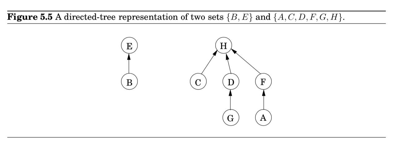
집합을 저장하는 방법 중 하나로 directed tree가 있음 (Figure 5.5)

• 
• 트리의 각 노드들은 집합의 원소
  • 특정 순서 없이 배열되어 있음
  • 각 노드는 parent pointers $\pi$ 를 가지고 있음
    • 이 parent pointers를 따라가면, tree의 root가 나옴
    • 이 root 원소를 집합의 $representative$ 혹은 $name$이라고 부름
    • 이 root 원소가 다른 원소들과 차이가 있는 부분은 parent pointer가 self-loop 형태임
  • 각 노드들은 $rank$를 가짐
    • 노드에 걸려 있는 subtree의 높이로 해석 가능

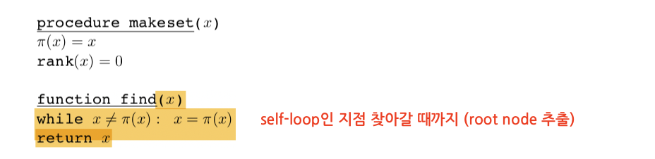
• $\texttt{makeset}$ : constant-time opeartion
• $\texttt{find}$ : parent pointers를 따라서 트리의 root까지 가므로, 트리의 높이에 비례하여 시간이 걸림

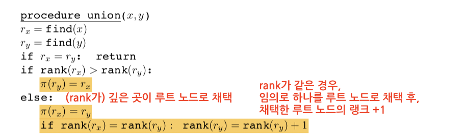
• $\texttt{union}$ : $union \; by \; rank$ scheme인 이유
  • for computational efficiency, choose a good strategy
    “$make\;the\;root\;of\;the\;shorter\;tree\;point\;to\;the\;root\;of\;the\;taller\;tree$”

Property 1 : For any $x$, $\text{rank}(x) < \text{rank}(\pi(x))$

• follows by induction
  • rank $k$인 루트 노트는 rank $k-1$인 루트를 가진 두 트리가 합쳐지면서 탄생함
• = 자기 부모보다는 랭크가 항상 낮다.

Property 2 : Any root node of rank $k$ has at least $2^k$ nodes in its tree.

• collorary : a node of rank $k$ has at least $2^k$ descendants.
  • 결국, 모든 노드들은 루트노드인 적이 한 번씩은 있었으며, 루트노드에서 탈출하면, 자신의 랭크 혹은 그것의 descendants 집합들 둘 다 변하지는 않음
  • 게다가, 서로 다른 rank-$k$ 노드들은 공통된 descendants를 가질 수 없음. (Property 1에 의해 어떤 원소든 rank $k$인 ancestor가 최대 1개를 가지고 있기 때문)

Property 3 : If there are $n$ elements overall, there can be at most $n/2^k$ nodes of rank $k$.

• 이 말은, 최대 rank가 $\log{n}$이라는 뜻임
• = 모든 트리들은 높이가 $\leq \log{n}$임
• = $\texttt{find}$와 $\texttt{union}$ 연산의 실행시간의 upper bound가 바로 $\log{n}$이 된다는 뜻

개인정리

• union의 종류는 2가지가 있음
  • Rank가 같은 트리가 합쳐지는 경우 = 한 쪽이 rank가 올라감
  • Rank가 다른 트리끼리 합쳐지는 경우 = 큰 rank가 먹어버림

Path compression

데이터 구조를 효율적으로 사용할 수 있는 방법은?

• 실제로 Kruskal’s algorithm total time
  = $O(|E| \log{|V|})$ for sorting edges + $O(|E| \log{|V|})$ for the $\texttt{union, find}$ operations
• (sorting 알고리즘이 $n\log{n}$, n=$|E|$이지만, $\log{|E|}\approx\log{|V|}$ 라고 할 수 있음)
• 이 때, 엣지들이 이미 sorting되어 있거나, weight가 작아서 충분히 linear time안에 수행가능하다면?
• 자료구조가 bottleneck이 될 것임
• 연산마다 $\log{n}$보다 더 좋은 성능을 내는 방법을 찾아봐야함.

어떻게 하면, $\log{n}$보다 좋은 $\texttt{union, find}$ 연산을 수행할 수 있을까?

• 정답은 자료구조를 좀 더 좋은 모양으로 가져가야 한다!

A randomized algorithm for minimum cut

5.1.5 Prim’s algorithm

• 다음과 같은 greedy schema를 따른 어떤 알고리즘이든 정합성이 보장됨
  $X = { } \texttt{(edges picked so far)}$
  $\texttt{repeat until } |X|=|V|-1:$
  $\;\;\;\; \texttt{pick a set } S \subset V \texttt{ for which } X \texttt{ has no edges between }S\texttt{ and }V-S$
  $\;\;\;\; \texttt{let } e \in E \texttt{ be the minimum-weight edge between }S\texttt{ and }V-S$
  $\;\;\;\; X = X \cup {e}$
• Kruskal’s alg. 말고도 Prim’s alg. 존재
  • edges $X$의 중간 집합은 항상 subtree
  • $S$는 이 subtree의 노드들의 집합으로 선택됨
  • 무슨 말?

Prim’s algorithm

• 각 iteration마다, $X$로 정의된 subtree는 한 개의 edge를 추가하면서 자라남
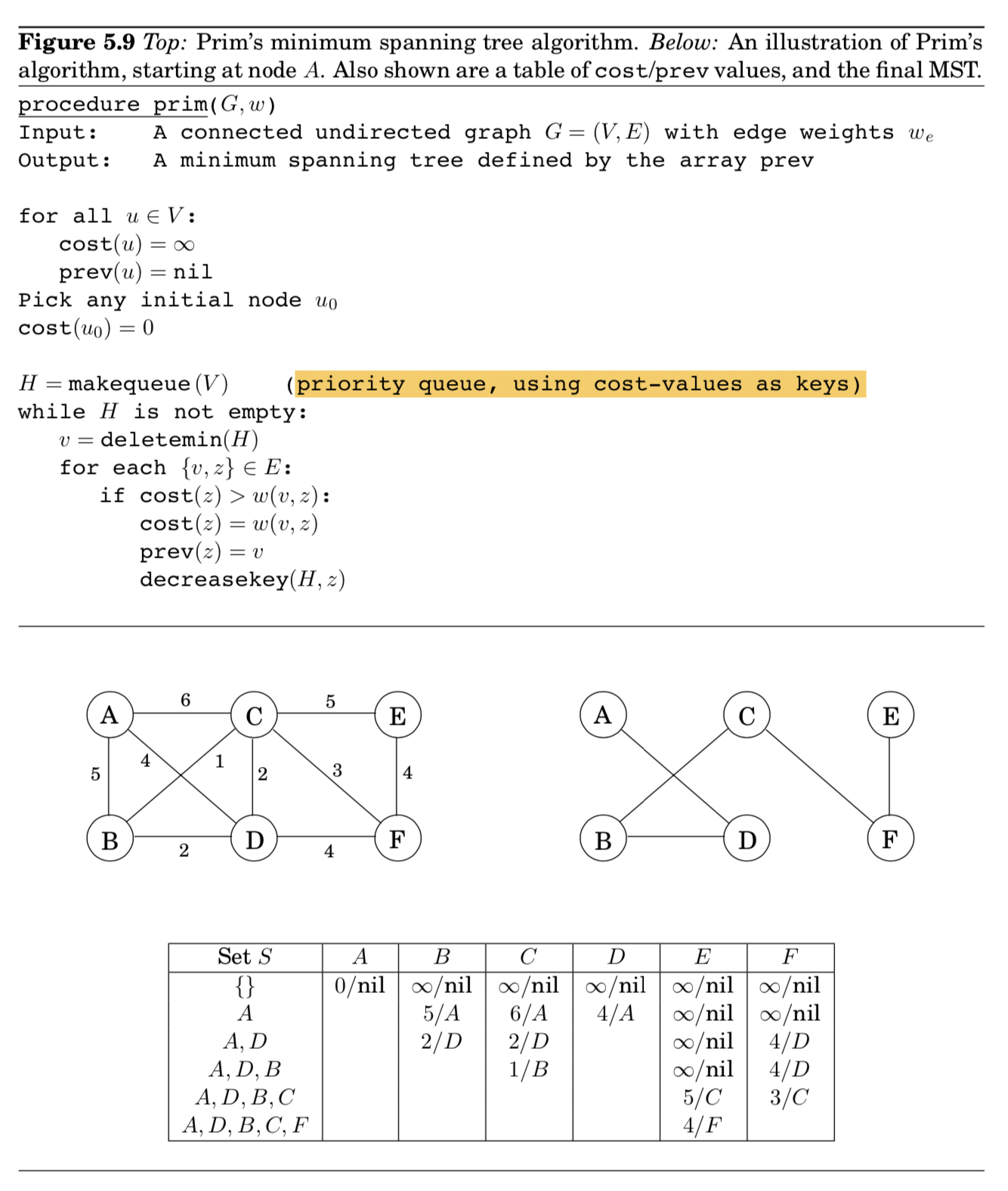
  • 노드 $v \notin S$를 $S$에 추가하는데, $\texttt{cost}(v) = {\min_{u\in{S}} w(u,v)}$를 최소화하는 비용으로
• Dijkstra’s alg과 굉장히 비슷
  • 차이를 보이는건, priority queue가 key values에 의해 정렬되어 있다는 것
  • node value에서 차이
    • Prim 알고리즘에서는, node의 value가 집합 $S$로부터 가장 가벼운 incoming edge의 가중치값임
    • 반면에, Dijkstra 알고리즘은 시작점으로부터 해당 노드까지의 전체 path의 길이임
  • 그럼에도, 같은 실행 시간 (depends on the particular priority queue implementation)
• final MST는 $\texttt{prev}$ 배열에 최종 저장됨

5.2 Huffman encoding

MP3 audio compression scheme에서, 음성 신호는 3가지 단계로 인코딩 됨

1. 일정 간격을 기준으로 샘플링하여 digitized됨. 실수값의 수열로 표현
   • 초마다 44,100개의 샘플을 뽑아낸다면
   • 50분동안 총 $T= 50 \times 60 \times \ 44,100 \approx 130 \text{ million}$
2. 실수 값을 가지는 각 샘플 $s_t$는 quantiezed됨.
   • finitie set $\Gamma$로부터 근방에 있는 숫자로 approximate
   • 이 때, 이 집합은 사람 귀로 구별할 수 있는 근사된 값의 나열로 표현
3. 길이가 $T$인 문자열은 binary로 인코딩 됨 ( $\Rightarrow$ Huffman encoding part)

Huffman encoding이 탄생한 이유

• 위의 예시로 살펴보자. ($T=130M$)
  • $\Gamma$ 집합은 총 4가지 값을 가지고 있고, 간략하게 기호로 $A,B,C,D$라고 하자.
  • $AACBAACDCAA…$와 같은 긴 길이의 문자열을 binary로 바꾸려면 어떻게 해야할까?
  • 가장 경제적인 방법은 각 기호를 2bits로 encoding 하는 것 (00, 10, 01, 11)
  • $\therefore$ 260 megabits are needed in total
• 우리가 더 나은 인코딩 방법을 찾을 수 있을까?
  • 더 자세히 살펴보니까 각 기호마다 frequency가 다름
  • $A$(70M), $B$(3M), $C$(20M), $D$(37M)
  • 자주 나오는 문자는 더 적은 bit로, 덜 나오는 문자는 좀 더 많은 bit로 표현한다면?
  • = {0, 01, 11, 001}와 같이 표현한다면?
  • 001의 표현이 애매할 수 있으니, prefix-free encoding을 사용하자.

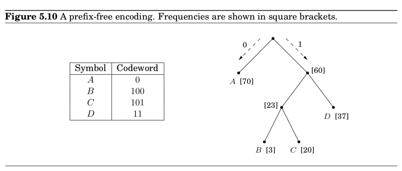
• $prefix-free$ property : no cdoeword can be aprefix of another codeword
• prefix-free encoding은 a full binary tree로 표현됨 (full = 모든 노드들은 자식이 없거나, 2개이거나) (Exercise 5.28)
  • (내 생각) 이 성질로 인해 depth가 하나씩 내려갈 때마다 두 노드 중 하나는 leaf로 끝낼 수 밖에 없음 (그림에서 0처럼)
    • 틀렸음
    • 그냥 트리구조의 leaf들은, prefix로 겹칠 수가 없음
• 이처럼 인코딩하니까, 17%의 개선효과가 있음 (213 megbaits)

Find OPT coding tree

• 주어진 $n$개의 기호 $f_1, f_2, …, f_n$ 에 대해서 최적의 트리는 어떻게 찾을 수 있을까?
• → leaves들이 모든 symbol을 대응시킬 수 있고, 인코딩의 전체 길이를 최소화하하는 트리를 찾으면 끝
  • 1) cost of tree = $\sum_{i=1}^n f_i \cdot (\text{depth of }i\text{th symbol in tree}) $
    • 예시) 70 * 1 + 37 *2 + 3 * 3 + 20 * 3 = 213
  • 2) cost of tree = sum of the frequencies of all leaves and internal nodes, except the root
    • 예시) leaves (70 + 37 + 3 + 20) + internal nodes (60 + 23) = 213
• 1) 식에 따라, 가장 적은 빈도수를 가진 2개의 symbols는 OPT tree의 bottom에 위치해야 함
• 이 방식을 greedily하게 접근하여 트리를 만들어갈 수 있음

Huffman (greedy)

• 1) 식에 따라
  • 가장 빈도수가 적은 2개의 symbols를 찾음, $f_1, f_2$이라고 간단히 가정
  • $f_1 + f_2$의 빈도수를 가진 새로운 노드를 만들고, 그 자식 노드로 $f_1, f_2$를 각각 배치
• 2) 식에 따라
  • 확정된 leaves $(f_1, f_2)$ + 나머지 트리 ($(f_1 + f_2), f_3, f_4, …, f_n$)
  • 뒤의 항인 나머지 트리는 다시 그 중에서 가장 작은 빈도수 두 개를 뽑는 구조로 순환시킬 수 있음
    • = frequencies list에서 $f_1, f_2$를 삭제하고, $(f_1+f_2)$를 삽입

이를 정리하면,

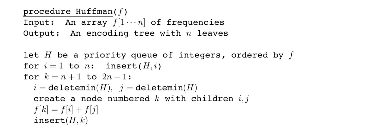
• priority queue로 표현
• takes $O(n\log{n})$ time if a binary heap is used (Section 4.5.2)

Entropy

• 3마리의 말에 대해 과거 200개의 경기를 보고, 확률분포(결과 4가지)로 요약함
• Q: Which horse is the most predictable?
  • look at compressibility
    • Huffman 알고리즘에 의해 200개의 값들을 인코딩해보면,
      Aurora : 200 * (0.15 * 2 + 0.10 * 3 + 0.70 * 1 + 0.05 * 3)
      Whirlwind : … = 380
      Phantasm : … = 420
    • Aurora가 가장 짧은 인코딩값을 가지므로, 가장 예측가능하다고 할 수 있음
• more compressible = less random = more predictable
  • $n$ 개의 가능한 결과들, 각각의 확률이 $p_1, p_2, … , p_n$ 임.
  • 분포로부터 $m$개의 나열된 시퀀스가 있다고 하면, $i$번째 결과는 $mp_i$번 등장할 것임 ($m$이 엄청 큰 경우)
  • 이를 좀 더 간결하게 나타내기 위해서, 각 확률들이 2의 지수승이라고 하자.
  • 또한, 모두 관측된 빈도값이라고 가정하자.
  • induction (Exercise 5.19)에 의해서, 이 시퀀스를 encoding하기 위해 필요한 bits 수는
    • $\sum_{i=1}^n mp_i \log{(1/p_i)}$ 임
  • 즉, 분포로부터 하나의 결과를 인코딩하기 위해 필요한 평균 bits 수는
    • $\sum_{i=1}^n p_i \log{(1/p_i)}$ 임
    • 이게 바로 분포의 $entropy$라고 볼 수 있고, 얼마나 랜덤성이 들어가있는지 측정하는 척도임
• 예시
  • fair coin entropy, $\frac{1}{2}\log{2} + \frac{1}{2}\log{2} = 1$
  • unfair coin entropy with $p_{H} = 3/4$, $\frac{3}{4}\log{\frac{4}{3}} + \frac{3}{4}\log{\frac{4}{3}} = 0.81$
  • 해석 : unfair coin이 fair coin보다 랜덤성이 덜 가미되어 있음, lower entropy

5.3 Horn fomulas

• for expressing logical facts and deriving conclusions
• The most objective object in a Horn formula is a $Boolean \; variable$
• In Horn formulas, knowledge about variables is represented by two kinds of $clauses$:
  • $Implications$
    • $(z \wedge w) \implies u $
  • $negative \; clauses$
    • $(\bar{u} \vee \bar{v} \vee \bar{y}$ )

GOAL : to determine whether there is a consistent explanation

• $satisfying \; assignment$ problem
• assignment of $\texttt{true/false}$ values to the variables that satisfies all the clauses.

Two directions for the two kinds of clauses

• 1) implications : set some of the variables to $\texttt{true}$
• 2) negative clauses : encourage us to make variables to $\texttt{false}$

Solving a Horn formula

• start with all variables $\texttt{false}$
• proceed to set some of them to $\texttt{true}$, one by one
  • implication check
    • $\texttt{while there is an implication that is not satisfied:}$
      $\;\;\;\; \texttt{set the right-hand variable of the implication to true}$
  • negative clauses check
    • $\texttt{if all pure negative clauses are satisfied: return the assignment}$
      $\texttt{else: return ‘‘formula is not satisfiable’’}$
• $\therefore$ actucally, greedy scheme

How efficient?

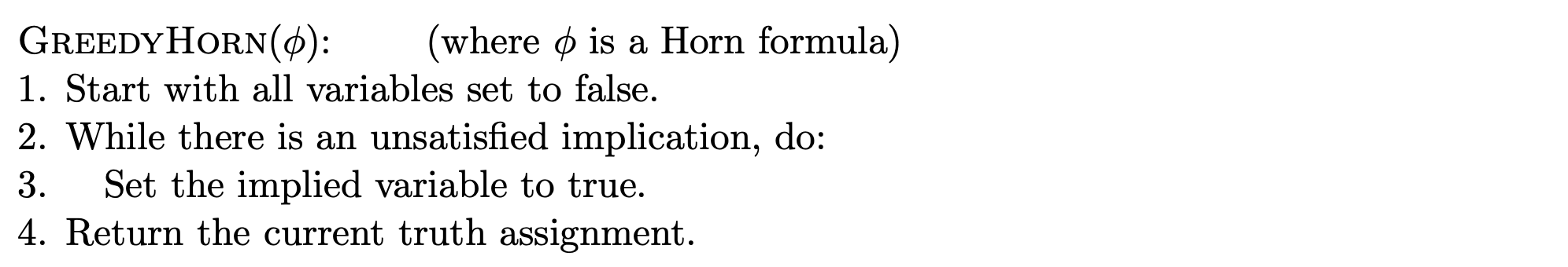
• GreedyHorn alg.
  • If the formula φ has length n, then GreedyHorn(φ) might require $O(n)$ iterations of the while loop, and each iteration of the while loop might take up to $O(n)$ work to scan for unsatisfied implications. Thus, GreedyHorn(φ) runs in $O(n^2)$ time: it is a quadratic-time algorithm.

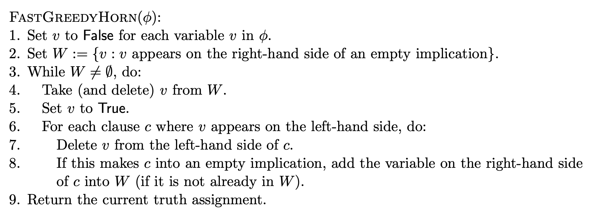
• FastGreedyHorn alg.
  • make linear time $O(n)$ (by David Wagner’s lecture note)

5.4 Set cover

문제 상황

• 각 점은 도시를 뜻하고, 각 도시를 어떤 학교에 배정될지를 정하는 문제
• 제한조건
  • 학교는 도시에 위치해 있어야 함
  • 일정 거리(ex. 30miles)를 넘어서면 사람들은 이동하지 않음
• 구하고 싶은것 : minimum number of schools needed
• $\Rightarrow$ 전형적인 $set \; cover$ 문제라고 볼 수 있음

문제 상황 (formally)

$\texttt{SET COVER} \
Input: \text{A set of elements } B; \text{ sets } S_1,…,S_m \subseteq B \
Output: \text{A selection of the } S_i \text{ whose union is }B. \
Cost: \text{Number of sets picked.}$

suggest a solution

• use greedy scheme
  • $\text{Repeat until all elements of }B\text{ are covered}:$
    $\text{Pick the set }S_i\text{ with the largest number of uncovered elements}$
• but not optimal in our situation
• But luckily, it isn’t too far from optimal

Claim : $B$가 $n$개의 원소들을 포함하고, 최적의 cover는 $k$개의 집합으로 구성되어 있다고 가정하자. 그러면 탐욕 알고리즘은 최대 $k\ln{n}$ 개의 집합들로 수행된다. ($k\ln{n}$ iterations)

pf) 탐욕 알고리즘을 $n$번 수행한 후에도 uncovered된 원소들의 수를 $n_t$라고 하자.
남은 원소들은 $k$개 의 optimal sets으로 covered되어야하기 때문에, 적어도 $n_t/k$ 개 크기의 cover set이 존재한다.
따라서 탐욕 전략에 의해 다음과 같은 수식을 만족하게 된다.
$n_{t+1} \leq n_t - \frac{n_t}{k} = n_t(1-\frac{1}{k})$
$\Rightarrow n_t \leq n_0(1-1/k)^t$
$\Rightarrow n_t \leq n_0(1-1/k)^t < n_0(e^{-1/k})^t = ne^{-t/k}$
$ (\because 1-x \leq e^{-x} \text{ for all }x)$
$t=k\ln{n}$이면, $n_t$가 1보다 작아지게 되므로, 더이상 cover할 원소가 남지 않는다.

결국, greedy alg. 과 optimal sol. 사이의 비율은 $\ln{n}$보다 항상 작게 된다.

• $\ln{n}$에 정말 가까워지게 되는 상황이 존재함 (Exercise 5.33)
• 이 최대치 비율인 $\ln{n}$을 탐욕알고리즘의 $approximation \; factor$라고 한다.

reference

• Union-find
  • https://bowbowbow.tistory.com/26#union-find-%EB%9E%80
• Amortized analysis for path compression
  • http://seclab.cs.sunysb.edu/sekar/cse548/ln/amort1.pdf
• Prim’s Algorithm
  • https://victorydntmd.tistory.com/102
• Huffman
  • https://hannom.tistory.com/36 / priority queue
• Horn formulas
  • http://people.cs.georgetown.edu/jthaler/ANLY550/lec7.pdf
  • https://people.eecs.berkeley.edu/~daw/teaching/cs170-s03/Notes/lecture15.pdf
• Set cover
  • https://huehak.tistory.com/218
  • http://web.cs.iastate.edu/~cs511/handout08/Set_cover.pdf